Principal Component Analysis(PCA)
Principal Component Analysis (PCA) is an unsupervised machine learning feature reduction technique for high-dimensional and correlated data sets. Images and text documents have high dimensional data sets which requires unnecessary computation power and storage. Basic goal of PCA is to select features which have high variance. High variance of a feature indicates more information it contributes. In this post, I will explain mathematical background of PCA and explore it step by step.
To understand PCA the following concepts are very important.
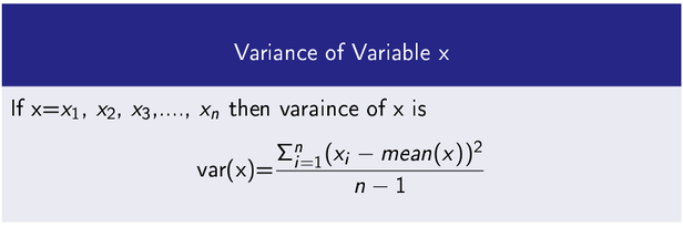
Variance
It measures how a data variable is scatter around its mean value.
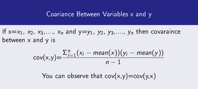
Covariance
It measures how two data variables vary with respect to each other.
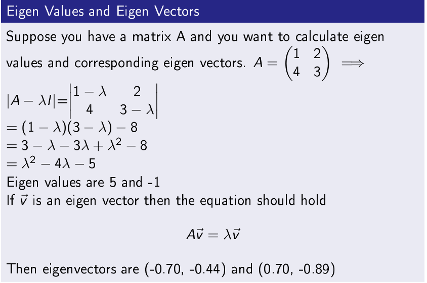
Eigenvalues and Eigenvectors
Steps is PCA
Input- A Dataset Having n Features x1, x2, x3,….,xn
Step-1
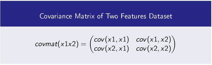
Find Covariance Matrix of Features
Step-2
Perform Eigen Decomposition of Symmetric Matrix
Step-3
Sort Eigen Values in Decreasing Order
Output- Order of Eigenvalues From High to Low Provides Principal Components
Dataset
To explore PCA, I have taken a dummy data set having 2 features (2 dimensional dataset) and 35 instances.
Two features x1 and x2 are
x1=[0.10,.15,.48,1.0,.34,.45,.10,.65,.9,0.10,-.12,0.2,1.0,0.5,-.6,.24,.12,.13,.9,.20,-.45,.86,.13,.15,.16,-.26,-.32,.47,-.34,.57,.26,.5,.9,.8,.12]
x2=[.15,.12,.45,.7,.1,-.05,-.16,.13,.20,-.02,.17,.12,.15,.12,-.19,.16,- .05,0.14,0.20,0.10,.5,.15,.18,.4,.7,.18,.1,.17,.3,0.08,.18,0.4,.15,.17,.10]
We will see that which feature is more important after applying PCA.
Step-1 Find Covariance Matrix of Dataset’s Features
In Python cov() function is used to compute covariance matrix.
And the following code produce the result
covmat=np.cov(x1x2)
print(‘Covariance Matrix\n’,covmat)
Covariance Matrix
[[0.17567513 0.01437941]
[0.01437941 0.03768235]]
Step-2 Perform Eigen Decomposition of Symmetric Matrix
A symmetric matrix has its all eigen values real and orthogonal eigenvectors.
The following code compute eigenvalues and eigenvectos in Python.
eigenval,eigenvec=egn.eig(covmat)
print(‘Eigenvalues\n’,eigenval)
print(‘Eigenvectors\n’,eigenvec)
Eigenvalues
[0.17715759 0.03619989]
Eigenvectors
[[ 0.99472755 -0.10255295]
[ 0.10255295 0.99472755]]
Step-3
Sort Eigenvalues in Decreasing Order
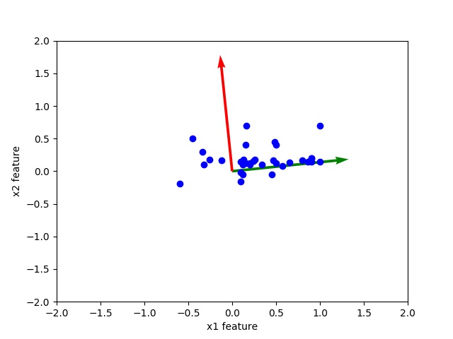
You can see the eigenvalues [0.17715759, 0.03619989] already in high to low order. Further, principal component corresponding to 0.17715759 is more significant than eigenvalue 0.03619989.
Observe the scatter plot of data and orthogonal eigen vectors. The corresponding high eigenvalues eigenvector is directed toward middle of data this shows that principal component corresponding to high eigen value is more important.
Python Code Code to Understand Principal Component Analysis(PCA)
import matplotlib.pyplot as plt
import numpy as np
from numpy import linalg as egn
fig = plt.figure()
ax = fig.gca()
x1=[0.10,.15,.48,1.0,.34,.45,.10,.65,.9,0.10,-.12,0.2,1.0,0.5,-.6,.24,.12,.13,.9,.20,-.45,.86,.13,.15,.16,-.26,-.32,.47,-.34,.57,.26,.5,.9,.8,.12]
x2=[.15,.12,.45,.7,.1,-.05,-.16,.13,.20,-.02,.17,.12,.15,.12,-.19,.16,-0.05,0.14,0.20,0.10,.5,.15,.18,.4,.7,.18,.1,.17,.3,0.08,.18,0.4,.15,.17,.10]
x1x2=np.array([x1,bx2])
covmat=np.cov(x1x2)
print(‘Covariance Matrix\n’,covmat)
eigenval,eigenvec=egn.eig(covmat)
print(‘Eigenvalues\n’,eigenval)
print(‘Eigenvectors\n’,eigenvec)
u,v=eigenvec
print(‘First Eigen Vector\n’,u)
print(‘Second Eigen Vector\n’,v)
x, y = ([0, 0],[0,0])
col=[‘g’,’r’]
ax.quiver(x, y, u,v,scale=3,color=col)
ax.set_ylim(-2, 2)
ax.set_xlim(-2, 2)
ax.scatter(x1, x2, c=’b’, marker=’o’)
ax.set_xlabel(‘x1 feature’)
ax.set_ylabel(‘x2 feature’)
plt.savefig(“PCA.jpg”)