Iris Classification Neural Network with Backpropagation
Bindeshwar Singh Kushwaha
PostNetwork Academy
Forward Propagation Step 1
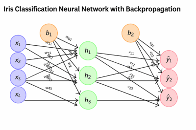
Dataset features:
\( x_1 = \text{Sepal length}, \; x_2 = \text{Sepal width}, \; x_3 = \text{Petal length}, \; x_4 = \text{Petal width} \)
Forward Propagation Step 2
\( z_{h1} = w_{11}x_1 + w_{21}x_2 + w_{31}x_3 + w_{41}x_4 + b_1 \)
Forward Propagation Step 3 (Sigmoid)
\( h_1 = \sigma(z_{h1}) = \frac{1}{1+e^{-z_{h1}}} \)
Forward Propagation Step 4
\( h_j = \sigma(z_{hj}), \quad j = 1,2,3 \)
Forward Propagation Step 5
\( z_{o1} = v_{11}h_1 + v_{21}h_2 + v_{31}h_3 + b_2 \)
Forward Propagation Step 6 (Softmax)
\( \hat y_j = \frac{e^{z_j}}{\sum_{k=1}^3 e^{z_k}}, \quad j=1,2,3 \)
Forward Propagation Step 7
\( \hat{\mathbf{y}} = (\hat y_1, \hat y_2, \hat y_3) \)
- Iris-setosa
- Iris-versicolor
- Iris-virginica
Forward Propagation Step 8 (Loss)
\( L = – \sum_{j=1}^3 y_j \log(\hat y_j) \)
Backpropagation Step 1
\( e_{o_j} = \hat y_j – y_j \)
Backpropagation Step 2
\( \frac{\partial L}{\partial v_{ij}} = h_i \cdot e_{o_j} \)
Backpropagation Step 3
\( e_{h_i} = \sigma'(z_{h_i}) \sum_j v_{ij} e_{o_j}, \quad \sigma'(z)=\sigma(z)(1-\sigma(z)) \)
Backpropagation Step 4
\( \frac{\partial L}{\partial w_{ki}} = x_k \cdot e_{h_i} \)
Backpropagation Step 5 (Weight Update)
\( w \leftarrow w – \eta \frac{\partial L}{\partial w} \)
Backpropagation Step 6 (Bias Update)
\( b_i \leftarrow b_i – \eta e_{h_i}, \quad b_j \leftarrow b_j – \eta e_{o_j} \)
Numerical Example: Setup
Input sample: \(x = (5.1, 3.5, 1.4, 0.2)\),
Target: \(y=(1,0,0)\),
Learning rate: \(\eta=0.1\)
Numerical Example: Initial Weights
\( W_1 = \begin{bmatrix}0.2 & -0.3 & 0.4\\ 0.1 & 0.2 & -0.2\\ 0.3 & -0.1 & 0.1\\ 0.2 & 0.4 & -0.3\end{bmatrix}, \;
b_1 = [0.1,0.2,0.1] \)
\( W_2 = \begin{bmatrix}0.1 & 0.2 & -0.1\\ -0.2 & 0.1 & 0.3\\ 0.05 & -0.1 & 0.2\end{bmatrix}, \;
b_2 = [0.1,0.05,0.2] \)
Hidden Layer Computation
\( z_h = x W_1 + b_1 \approx [0.93, -0.08, 0.34] \)
\( h = \sigma(z_h) \approx [0.716, 0.480, 0.584] \)
Output Layer Computation
\( z = hW_2 + b_2 = [0.237, 0.325, 0.441] \)
\(\hat{y}_i = \frac{e^{z_i}}{\sum_{j=1}^3 e^{z_j}}\)
\(\hat y = [0.317, 0.331, 0.352]\)
Loss Computation
\( L = -\sum_j y_j \log(\hat y_j) \approx 1.148 \)
Output Error
\( e_o = \hat y – y \approx [-0.683, 0.331, 0.352] \)
\( \frac{\partial L}{\partial W_2} = h^T e_o^T \)
Hidden Layer Error
\( e_h = (e_o W_2^T) \odot h \odot (1-h) \approx [-0.0097, 0.011, 0.0117] \)
\( \frac{\partial L}{\partial W_1} = x^T e_h \)
Weight Update Numerical Example
\( W_1 \leftarrow W_1 – \eta \frac{\partial L}{\partial W_1}, \;
W_2 \leftarrow W_2 – \eta \frac{\partial L}{\partial W_2} \)
\( b_1 \leftarrow b_1 – \eta e_h, \;
b_2 \leftarrow b_2 – \eta e_o \)
Summary of Steps
- Forward pass: compute \(z_h, h, z_o, \hat y\)
- Compute loss: cross-entropy
- Backprop: compute \(e_o, e_h\)
- Update weights and biases
- Repeat until convergence