Correlation
Correlation measures the relation between two variables that how they are related. And is denoted by r and ρ moreover, the correlation quantifies the level of relationship between -1 to +1. If the value of correlation r is -1 then there is perfect negative relationship. If value of correlation is +1 then there is positive correlation between variables.
Important Points
- r=-1 Perfect Negative Correlation
- r=0 No Correlation
- r=1 Perfect Positive Correlation
- r lies between -1 and +1
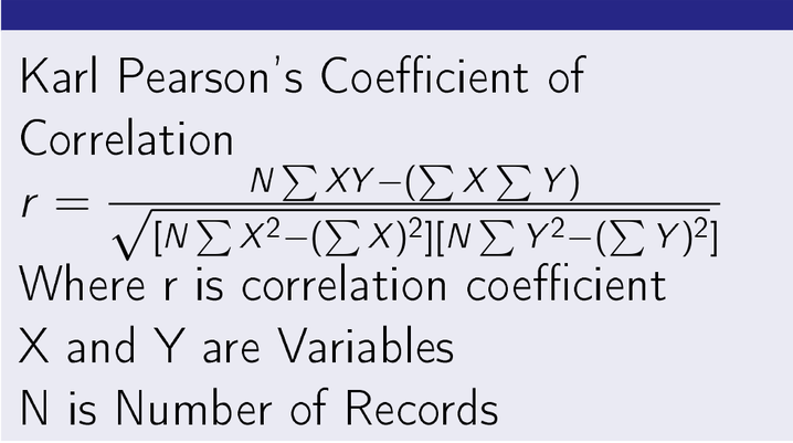
Pearson Correlation-
Named after Karl Pearson it is the most widely used formula for correlation coefficient. If there are two variables X and Y having N instances. Then the correlation coefficient r is given in formula.
Calculation of Pearson’s Correlation Coefficient in Python
Let there be two variables X and Y
The values of X and Y are
X = [40,46,55,60,70,75,78,80 , 85, 95]
Y = [40,46,55,60,70,75, 78,80 , 85, 95]
Then Python’s code for computation of correlation is
#Computation of Pearson’s Correlation Coefficient
from scipy.stats import pearsonr
from matplotlib import pyplot
X = [40,46,55,60,70,75,78,80 , 85, 95]
Y = [40,46,55,60,70,75, 78,80 , 85, 95]
# pearsonr(X,Y) Calculates Pearson’s Correlation Coefficient
r= pearsonr(X,Y)
print(“Pearson’s Correlation Coefficient”, r)
pyplot.scatter(X,Y)
pyplot.savefig(“pearsonr.png”)
The output of the program would be
Output: Pearson’s Correlation Coefficient (1.0, 0.0)
Scatter plot for the data is
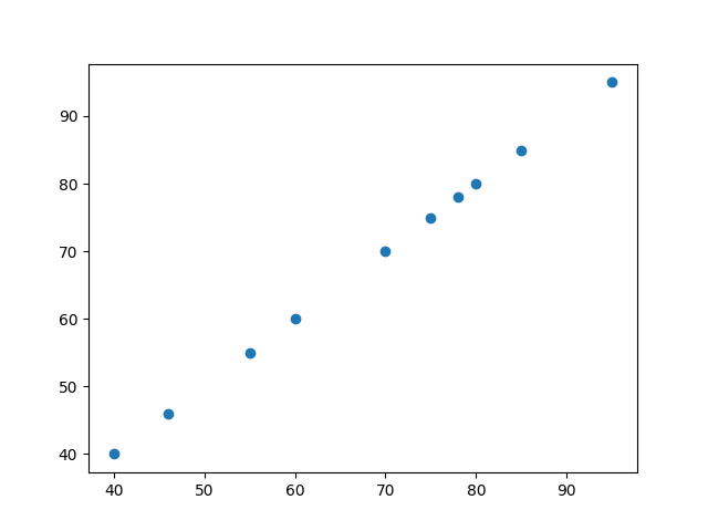
From the above scatter diagram you can observed that there is perfect positive correlation between X and Y variables.
This is due to X and Y having the same values.
Again consider the data set
X = [40,46,55,60,70,75,78,80 , 85, 95]
Y= [95,85,80,78,75,70,60,55,46,40]
And Corresponding Python’s Code
#Computation of Pearson’s Correlation Coefficient
from scipy.stats import pearsonr
from matplotlib import pyplot
X = [40,46,55,60,70,75,78,80 , 85, 95]
Y= [95,85,80,78,75,70,60,55,46,40]
# pearsonr(X,Y) Calculates Pearson’s Correlation Coefficient
r= pearsonr(X,Y)
print(“Pearson’s Correlation Coefficient”, r)
pyplot.scatter(X,Y)
pyplot.savefig(“negativepearsonr.png”)
The output of the program would be
Pearson’s Correlation Coefficient (-0.9613416714042071, 9.325227687014438e-06)
The the scatter plot of the data is
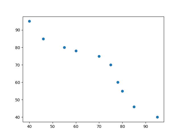
You can observed that I have just reversed the data and then relation has become negatively correlated.
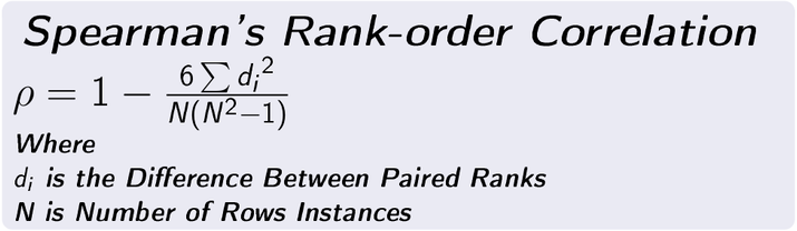
Spearman Rank Correlation
Spearman’n rank correlation is used for qualitative data. The first step is to convert qualitative comparative data into rank. Then apply the following formula.
 Let R1 and R2 be ranks given to statistics and mathematics students in a university.
Set of values of R1 and R2 are
R1 = [3,5,8,10,15,26,30,36,40,42]
R2 = [3,5,8,10,15,26,30,36,40,42]
Python’s Code for Calculation Spearman’s Rank Correlation Coefficient
#Spearman’s Correlation Coefficient
from scipy.stats import spearmanr
from matplotlib import pyplot
R1 = [3,5,8,10,15,26,30,36,40,42]
R2 = [3,5,8,10,15,26,30,36,40,42]
# spearmanr(R1,R2) Calculates Spearman’s Rank Correlation Coefficient
r= spearmanr(R1,R2)
print(“Spearman’s Correlation Coefficient”, r)
pyplot.scatter(R1,R2)
pyplot.savefig(“spearmanr.png”)
Output of the program would be
Output : Spearman’s Correlation Coefficient SpearmanrResult(correlation=0.9999999999999999, pvalue=6.646897422032013e-64)
And scatter plot is
 I have taken R1 and R2 having the same that is why there is perfect positive correlation.
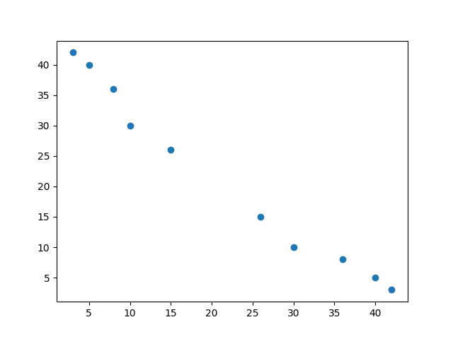
Furthermore, If I reverse R2 then the plot will be
The Python’s code is
#Spearman’s Correlation Coefficient
from scipy.stats import spearmanr
from matplotlib import pyplot
R1 = [3,5,8,10,15,26,30,36,40,42]
R2= [42,40,36,30,26,15,10,8,5,3]
# spearmanr(R1,R2) Calculates Spearman’s Rank Correlation Coefficient
r= spearmanr(R1,R2)
print(“Spearman’s Correlation Coefficient”, r)
pyplot.scatter(R1,R2)
pyplot.savefig(“negcorspearmanr.png”)
The output of the program would be
Output : Spearman’s Correlation Coefficient SpearmanrResult(correlation=-0.9999999999999999, pvalue=6.646897422032013e-64)
And corresponding scatter plot is
 Conclusion-
Correlation is very important topic in machine learning, statistics and data science. It helps to find out relationship in a data set. In this post, I have explained two popular method for correlation computation. Hope you will understand and apply.
References-
- Meng, X.L., Rosenthal, R. and Rubin, D.B., 1992. Comparing correlated correlation coefficients. Psychological bulletin, 111(1), p.172.
- Bansal, N., Blum, A. and Chawla, S., 2004. Correlation clustering. Machine learning, 56(1-3), pp.89-113. https://link.springer.com/content/pdf/10.1023/B:MACH.0000033116.57574.95.pdf