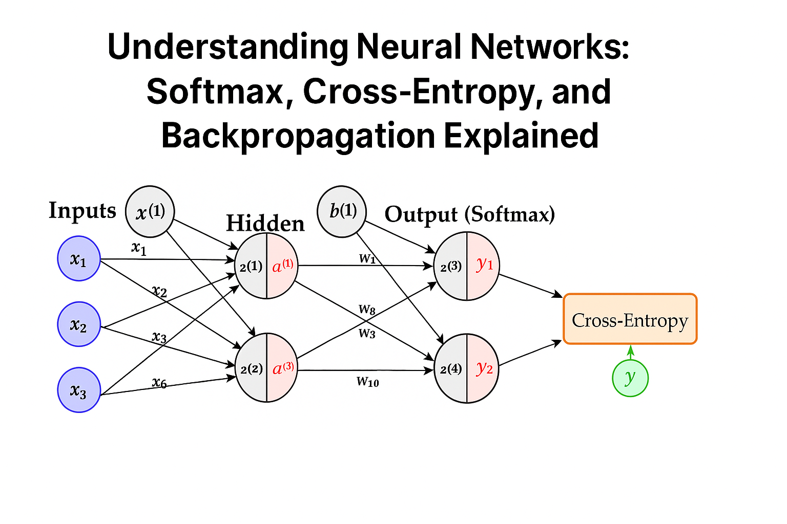
Neural Network with Softmax + Cross-Entropy

• Input Layer: The network receives 3 input features, denoted \(x_1, x_2, x_3\).
• Hidden Layer: 2 neurons in the hidden layer with activations \(a^{(1)}\) and \(a^{(2)}\).
• Output Layer: 2 outputs \(z^{(3)}, z^{(4)}\), passed through softmax.
• Softmax Activation: Converts outputs into probability predictions \(\hat{y}_1, \hat{y}_2\).
• Loss Function: Cross-Entropy Loss compares predicted outputs \(\hat{y}\) with true labels \(y\).

Step 1: Hidden Pre-Activation

Given inputs:

\(x_1=1, \; x_2=2, \; x_3=-1\)
\(w_1=0.2, \; w_2=-0.3, \; w_3=0.4, \; b^{(1)}=0.5\)
\(w_4=-0.5, \; w_5=0.1, \; w_6=0.2\)

\(z^{(1)} = 0.2(1) – 0.3(2) + 0.4(-1) + 0.5 = -0.3\)
\(z^{(2)} = -0.5(1) + 0.1(2) + 0.2(-1) + 0.5 = 0\)

Step 2: Hidden Activation (Sigmoid)

\(a^{(1)} = \sigma(z^{(1)}) = \dfrac{1}{1+e^{0.3}} \approx 0.426\)
\(a^{(2)} = \sigma(z^{(2)}) = \dfrac{1}{1+e^0} = 0.5\)

Step 3: Output Pre-Activation

\(w_7=0.3,\; w_8=-0.1,\; w_9=0.4,\; w_{10}=0.2,\; b^{(2)}=0.1\)

\(z^{(3)} = 0.3(0.426) + 0.4(0.5) + 0.1 \approx 0.428\)
\(z^{(4)} = -0.1(0.426) + 0.2(0.5) + 0.1 \approx 0.185\)

Step 4: Output Activation (Softmax)

\(\hat{y}_1 = \dfrac{e^{0.428}}{e^{0.428}+e^{0.185}} \approx 0.561\)
\(\hat{y}_2 = \dfrac{e^{0.185}}{e^{0.428}+e^{0.185}} \approx 0.439\)

Step 5: Cross-Entropy Loss

\(L = -\sum_{i=1}^2 y_i \ln(\hat{y}_i)\)
For \(y=[1,0]\):
\(L = -(1 \cdot \ln(0.561)) \approx 0.579\)

Step 6–13: Backpropagation (Gradients)

Using the chain rule:

\(\dfrac{\partial L}{\partial w_7} = (\hat{y}_1 – y_1)a^{(1)}\)
\(\dfrac{\partial L}{\partial w_8} = (\hat{y}_1 – y_1)a^{(2)}\)
\(\dfrac{\partial L}{\partial w_9} = (\hat{y}_2 – y_2)a^{(1)}\)
\(\dfrac{\partial L}{\partial w_{10}} = (\hat{y}_2 – y_2)a^{(2)}\)

Weight Update Rule

Using gradient descent with learning rate \(\eta\):

\(w \leftarrow w – \eta \dfrac{\partial L}{\partial w}\)

Example:
\(w_7 \leftarrow w_7 – \eta (\hat{y}_1 – y_1)a^{(1)}\)
\(w_8 \leftarrow w_8 – \eta (\hat{y}_1 – y_1)a^{(2)}\)

Backpropagation into Input Weights

For hidden neuron 1:
\(\dfrac{\partial L}{\partial w_1} = \big[(\hat{y}_1 – y_1)w_7 + (\hat{y}_2 – y_2)w_9\big] \, a^{(1)}(1-a^{(1)}) \, x_1\)

Similarly, gradients for \(w_2, w_3, w_4, w_5, w_6\) follow the same pattern.

PDF

Video