Neural Network Architecture for Iris Dataset

Author: Bindeshwar Singh Kushwaha
Institution: PosstNetwork Academy

 Outline

• Iris Dataset Overview
• Neural Network Architecture
• Mathematical Formulation
• Code Walkthrough
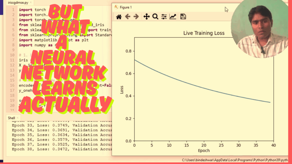
• Live Loss Plot
• Evaluation and Summary

 Sample from Iris Dataset

Sepal Length	Sepal Width	Petal Length	Petal Width	Class
5.1	3.5	1.4	0.2	Setosa
6.2	2.9	4.3	1.3	Versicolor
5.9	3.0	5.1	1.8	Virginica

 Neural Network Design

• Input Layer: 4 neurons (sepal/petal length/width)
• Hidden Layer: 10 neurons with ReLU
• Output Layer: 3 neurons (Setosa, Versicolor, Virginica)

📊 Mathematical Formulation

1. Mean Squared Error (MSE) Loss:

$$
\text{Loss} = \frac{1}{N} \sum_{i=1}^{N} (y_i – \hat{y}_i)^2
$$

2. Stochastic Gradient Descent (SGD) Update:

$$
\theta_{t+1} = \theta_t – \eta \cdot \nabla_{\theta} J(\theta)
$$

3. Xavier Initialization:

$$
W \sim \mathcal{U}\left(-\frac{\sqrt{6}}{\sqrt{n_{in} + n_{out}}}, \frac{\sqrt{6}}{\sqrt{n_{in} + n_{out}}}\right)
$$

💻 PyTorch Code Walkthrough

1. Import Libraries and Load Data

import torch
import torch.nn as nn
import torch.optim as optim
from sklearn.datasets import load_iris
from sklearn.model_selection import train_test_split
from sklearn.preprocessing import StandardScaler, OneHotEncoder
import matplotlib.pyplot as plt
import numpy as np

iris = load_iris()
X = iris.data
y = iris.target.reshape(-1, 1)

encoder = OneHotEncoder(sparse_output=False)
y_onehot = encoder.fit_transform(y)

scaler = StandardScaler()
X = scaler.fit_transform(X)

2. Convert to Tensors and Split Data

X = torch.tensor(X, dtype=torch.float32)
y_onehot = torch.tensor(y_onehot, dtype=torch.float32)

X_train, X_test, y_train, y_test = train_test_split(
    X, y_onehot, test_size=0.2, random_state=42)

3. Define Neural Network

class IrisNet(nn.Module):
    def __init__(self):
        super(IrisNet, self).__init__()
        self.fc1 = nn.Linear(4, 10)
        self.relu = nn.ReLU()
        self.fc2 = nn.Linear(10, 3)

    def forward(self, x):
        x = self.relu(self.fc1(x))
        x = self.fc2(x)
        return x

model = IrisNet()

4. Xavier Weight Initialization

def init_weights(m):
    if isinstance(m, nn.Linear):
        nn.init.xavier_uniform_(m.weight)
        nn.init.zeros_(m.bias)

model.apply(init_weights)

5. Loss and Optimizer

criterion = nn.MSELoss()
optimizer = optim.SGD(model.parameters(), lr=0.01)

6. Live Plot Setup

plt.ion()
fig, ax = plt.subplots()
losses = []
line, = ax.plot(losses)
ax.set_xlim(0, 100)
ax.set_ylim(0, 2)
ax.set_xlabel("Epoch")
ax.set_ylabel("Loss")
ax.set_title("Live Training Loss")

✅ Summary

• Trained a 3-layer neural net on the Iris dataset using PyTorch
• Used SGD optimizer with MSE loss
• Employed Xavier initialization
• Live loss plotting during training

PDF

iris_pytorch_beamer

Videos