Contents
hide
Normal Distribution
A Detailed Step-by-Step Explanation
By Bindeshwar Singh Kushwaha
PostNetwork Academy
Introduction: Random Variables
- A random variable (r.v.) is a function that assigns a numerical value to each outcome of a random experiment.
- There are two main types of random variables:
- Discrete Random Variable: Takes countable values (e.g., number of heads in 3 coin tosses).
- Continuous Random Variable: Takes any value in an interval of real numbers (e.g., height, weight, time).
- In this section, we focus on the Continuous Random Variable and the most important one: the Normal Distribution.
Definition: Continuous Random Variable
- A random variable \( X \) is said to be continuous if it can take any real value in an interval.
- Its probability is described by a Probability Density Function (PDF) \( f(x) \).
- The probability that \( X \) lies between \( a \) and \( b \) is:
\( P(a < X < b) = \int_a^b f(x)\,dx \)
- The total area under the curve is always 1:
\( \int_{-\infty}^{\infty} f(x)\,dx = 1 \)
- The most common continuous distribution is the Normal Distribution.
Definition: Normal Distribution
-
- A continuous random variable \( X \) follows a Normal Distribution with mean \( \mu \) and variance \( \sigma^2 \) if its PDF is:
\( f(x) = \frac{1}{\sigma \sqrt{2\pi}} e^{ -\frac{(x – \mu)^2}{2\sigma^2} }, \quad -\infty < x < \infty \)
- It is denoted as \( X \sim N(\mu, \sigma^2) \).
- The curve is symmetric about the mean \( \mu \).
- The spread (width) depends on the standard deviation \( \sigma \).
Standard Normal Distribution
-
- If \( X \sim N(\mu, \sigma^2) \), we define a new variable:
\( Z = \frac{X – \mu}{\sigma} \)
- Then \( Z \) follows the Standard Normal Distribution:
\( Z \sim N(0, 1) \)
- Its PDF is given by:
\( f(z) = \frac{1}{\sqrt{2\pi}} e^{-z^2/2} \)
- This is the most commonly used form for normal probability tables.
Properties of Normal Distribution
-
- Mean: \( E[X] = \mu \)
- Variance: \( \text{Var}(X) = \sigma^2 \)
- Shape:
- Bell-shaped and symmetric about \( \mu \)
- Mean = Median = Mode
- Area under the curve = 1
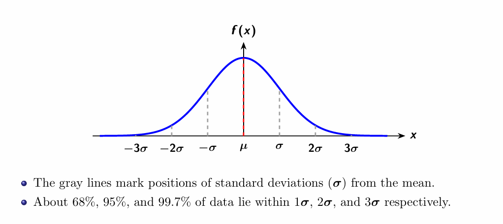
- Empirical Rule:
\[
\begin{array}{lcl}
\text{Within } 1\sigma &\Rightarrow& 68.27\% \\
\text{Within } 2\sigma &\Rightarrow& 95.45\% \\
\text{Within } 3\sigma &\Rightarrow& 99.73\%
\end{array}
\]
\begin{array}{lcl}
\text{Within } 1\sigma &\Rightarrow& 68.27\% \\
\text{Within } 2\sigma &\Rightarrow& 95.45\% \\
\text{Within } 3\sigma &\Rightarrow& 99.73\%
\end{array}
\]
Graph of Normal Distribution
PDF
NormalDistDef
Applications of Normal Distribution
- Used in natural and social sciences to represent real-valued random variables.
- Commonly applied in:
- Measurement errors
- Heights, weights, and blood pressure
- Quality control and industrial processes
- Finance (returns, risk modeling)
- The Central Limit Theorem states that the sum of many independent random variables tends to a normal distribution.
Reach PostNetwork Academy
- Website: www.postnetwork.co
- YouTube Channel: PostNetwork Academy
- Facebook Page: facebook.com/postnetworkacademy
- LinkedIn Page: linkedin.com/company/postnetworkacademy
- GitHub Repositories: github.com/postnetworkacademy